01 Oct 2020

Analysis: Air Quality in India

Let’s explore air quality data of India. This dataset has daily pollutant readings for the period 2015-2020.

Goal of this analysis:

Understand how is the trend of these pollutants over the years
How are the two-tier cities coping up with the increased level of infrastructure development and vehicular pollution due to increased human migration.

Source of the Data:

https://www.kaggle.com/rohanrao/air-quality-data-in-india?select=city_day.csv

Process of calculating air quality index:

https://www.kaggle.com/rohanrao/calculating-aqi-air-quality-index-tutorial

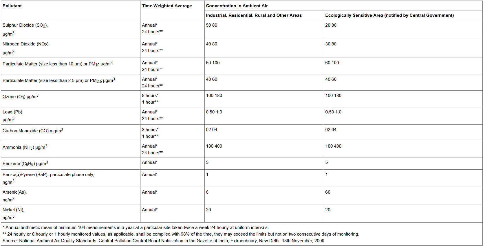
What are the safe limits of these pollutants in air for India?

http://www.arthapedia.in/index.php?title=Ambient_Air_Quality_Standards_in_India

About the Dataset:

The dataset has air quality readings of major India cities for the period 2015-2020.
This dataset captures the air quality parameters of PM2.5, PM10, Nitrogen Oxide (NO), Nitrogen Dioxide (NO2), Ammonia (NH3), Carbon Monoxide (CO), Sulphur Dioxide (SO2), Ozone (O3), Benzene, Toulene, Xylene.
Computed Air Quality Index included in the dataset
Population estimates of these cities were collected separately and added to the dataset to understand the role of population on air quality.

Load Datasets

Load Pollution and Population Estimates datasets.

# Load pollution data
pollution <- read.csv('https://raw.githubusercontent.com/learning-monk/datasets/master/ENVIRONMENT/Indian_cities_daily_pollution_2015-2020.csv', 
                      stringsAsFactor=FALSE, na.strings=c(""))

# Load population estimates data
pop_est <- read.csv('https://raw.githubusercontent.com/learning-monk/datasets/master/ENVIRONMENT/cities%20with%20population%20estimates%202019.csv',
                   stringsAsFactor=FALSE)

# Let's see the structure of the dataset
str(pollution)

## 'data.frame':    29531 obs. of  16 variables:
##  $ City      : chr  "Ahmedabad" "Ahmedabad" "Ahmedabad" "Ahmedabad" ...
##  $ Date      : chr  "2015-01-01" "2015-01-02" "2015-01-03" "2015-01-04" ...
##  $ PM2.5     : num  NA NA NA NA NA NA NA NA NA NA ...
##  $ PM10      : num  NA NA NA NA NA NA NA NA NA NA ...
##  $ NO        : num  0.92 0.97 17.4 1.7 22.1 ...
##  $ NO2       : num  18.2 15.7 19.3 18.5 21.4 ...
##  $ NOx       : num  17.1 16.5 29.7 18 37.8 ...
##  $ NH3       : num  NA NA NA NA NA NA NA NA NA NA ...
##  $ CO        : num  0.92 0.97 17.4 1.7 22.1 ...
##  $ SO2       : num  27.6 24.6 29.1 18.6 39.3 ...
##  $ O3        : num  133.4 34.1 30.7 36.1 39.3 ...
##  $ Benzene   : num  0 3.68 6.8 4.43 7.01 5.42 0 0 0 0 ...
##  $ Toluene   : num  0.02 5.5 16.4 10.14 18.89 ...
##  $ Xylene    : num  0 3.77 2.25 1 2.78 1.93 0 0 0 0 ...
##  $ AQI       : int  NA NA NA NA NA NA NA NA NA NA ...
##  $ AQI_Bucket: chr  NA NA NA NA ...

# Convert date column to Date format
pollution$Date <- as.Date(pollution$Date)

Merge population estimates and pollution datasets into a Combined dataset

combined <- merge(pollution, pop_est, by = "City")
str(combined)

## 'data.frame':    29531 obs. of  21 variables:
##  $ City                         : chr  "Ahmedabad" "Ahmedabad" "Ahmedabad" "Ahmedabad" ...
##  $ Date                         : Date, format: "2015-01-01" "2015-01-02" ...
##  $ PM2.5                        : num  NA NA NA NA NA NA NA NA NA NA ...
##  $ PM10                         : num  NA NA NA NA NA NA NA NA NA NA ...
##  $ NO                           : num  0.92 0.97 17.4 1.7 22.1 ...
##  $ NO2                          : num  18.2 15.7 19.3 18.5 21.4 ...
##  $ NOx                          : num  17.1 16.5 29.7 18 37.8 ...
##  $ NH3                          : num  NA NA NA NA NA NA NA NA NA NA ...
##  $ CO                           : num  0.92 0.97 17.4 1.7 22.1 ...
##  $ SO2                          : num  27.6 24.6 29.1 18.6 39.3 ...
##  $ O3                           : num  133.4 34.1 30.7 36.1 39.3 ...
##  $ Benzene                      : num  0 3.68 6.8 4.43 7.01 5.42 0 0 0 0 ...
##  $ Toluene                      : num  0.02 5.5 16.4 10.14 18.89 ...
##  $ Xylene                       : num  0 3.77 2.25 1 2.78 1.93 0 0 0 0 ...
##  $ AQI                          : int  NA NA NA NA NA NA NA NA NA NA ...
##  $ AQI_Bucket                   : chr  NA NA NA NA ...
##  $ State                        : chr  "Gujarat" "Gujarat" "Gujarat" "Gujarat" ...
##  $ Part_of_India                : chr  "West India" "West India" "West India" "West India" ...
##  $ Metropolitan_Area            : int  1 1 1 1 1 1 1 1 1 1 ...
##  $ Population_as_per_2011_census: int  5570585 5570585 5570585 5570585 5570585 5570585 5570585 5570585 5570585 5570585 ...
##  $ Population_Estimate_2019     : int  8644400 8644400 8644400 8644400 8644400 8644400 8644400 8644400 8644400 8644400 ...

# Convert newly added columns to factors
combined$State <- as.factor(combined$State)
combined$Part_of_India <- as.factor(combined$Part_of_India)
combined$Metropolitan_Area <- as.factor(combined$Metropolitan_Area)

# Convert City and AQI_Bucket to factor variables and Date column to Date
combined$City <- as.factor(combined$City)
combined$AQI_Bucket <- as.factor(combined$AQI_Bucket)
combined$Date <- as.Date(combined$Date, format = '%Y-%m-%d')

# Add Month and Year to combined
combined$Month <- as.factor(format(combined$Date, '%b'))
combined$Year <- as.factor(as.numeric(format(combined$Date, '%Y')))

# Re-order Month Values
combined$Month <- factor(combined$Month, levels = c('Jan', 'Feb', 'Mar', 'Apr', 'May', 'Jun', 'Jul', 'Aug', 'Sep',
                                                     'Oct', 'Nov', 'Dec'))
str(combined)

## 'data.frame':    29531 obs. of  23 variables:
##  $ City                         : Factor w/ 26 levels "Ahmedabad","Aizawl",..: 1 1 1 1 1 1 1 1 1 1 ...
##  $ Date                         : Date, format: "2015-01-01" "2015-01-02" ...
##  $ PM2.5                        : num  NA NA NA NA NA NA NA NA NA NA ...
##  $ PM10                         : num  NA NA NA NA NA NA NA NA NA NA ...
##  $ NO                           : num  0.92 0.97 17.4 1.7 22.1 ...
##  $ NO2                          : num  18.2 15.7 19.3 18.5 21.4 ...
##  $ NOx                          : num  17.1 16.5 29.7 18 37.8 ...
##  $ NH3                          : num  NA NA NA NA NA NA NA NA NA NA ...
##  $ CO                           : num  0.92 0.97 17.4 1.7 22.1 ...
##  $ SO2                          : num  27.6 24.6 29.1 18.6 39.3 ...
##  $ O3                           : num  133.4 34.1 30.7 36.1 39.3 ...
##  $ Benzene                      : num  0 3.68 6.8 4.43 7.01 5.42 0 0 0 0 ...
##  $ Toluene                      : num  0.02 5.5 16.4 10.14 18.89 ...
##  $ Xylene                       : num  0 3.77 2.25 1 2.78 1.93 0 0 0 0 ...
##  $ AQI                          : int  NA NA NA NA NA NA NA NA NA NA ...
##  $ AQI_Bucket                   : Factor w/ 6 levels "Good","Moderate",..: NA NA NA NA NA NA NA NA NA NA ...
##  $ State                        : Factor w/ 20 levels "Andhra Pradesh",..: 4 4 4 4 4 4 4 4 4 4 ...
##  $ Part_of_India                : Factor w/ 6 levels "Central India",..: 6 6 6 6 6 6 6 6 6 6 ...
##  $ Metropolitan_Area            : Factor w/ 2 levels "0","1": 2 2 2 2 2 2 2 2 2 2 ...
##  $ Population_as_per_2011_census: int  5570585 5570585 5570585 5570585 5570585 5570585 5570585 5570585 5570585 5570585 ...
##  $ Population_Estimate_2019     : int  8644400 8644400 8644400 8644400 8644400 8644400 8644400 8644400 8644400 8644400 ...
##  $ Month                        : Factor w/ 12 levels "Jan","Feb","Mar",..: 1 1 1 1 1 1 1 1 1 1 ...
##  $ Year                         : Factor w/ 6 levels "2015","2016",..: 1 1 1 1 1 1 1 1 1 1 ...

# Find missing values in the dataset
na_count <-sapply(combined, function(y) sum(length(which(is.na(y)))))
na_count <- data.frame(na_count)
na_count

##                               na_count
## City                                 0
## Date                                 0
## PM2.5                             4598
## PM10                             11140
## NO                                3582
## NO2                               3585
## NOx                               4185
## NH3                              10328
## CO                                2059
## SO2                               3854
## O3                                4022
## Benzene                           5623
## Toluene                           8041
## Xylene                           18109
## AQI                               4681
## AQI_Bucket                        4681
## State                                0
## Part_of_India                        0
## Metropolitan_Area                    0
## Population_as_per_2011_census        0
## Population_Estimate_2019             0
## Month                                0
## Year                                 0

Except City and Date columns, rest of the columns have NAs. Let’s not impute these missing values as they are not evenly missing. We will ignore these values in the plots for now.

# Re-order bucket values in logical order in AQI_Bucket columns
combined$AQI_Bucket <- factor(combined$AQI_Bucket, levels = c('Severe', 'Very Poor', 'Poor', 'Moderate',
                                                               'Satisfactory', 'Good'))

# How is AQI_Bucket distributed?
table(combined[!is.na('AQI_Bucket'), 'AQI_Bucket'])

## 
##       Severe    Very Poor         Poor     Moderate Satisfactory         Good 
##         1338         2337         2781         8829         8224         1341

# Plot the distribution of AQI levels
library(ggplot2)

ggplot(subset(combined, !is.na(AQI_Bucket)), aes(x=AQI_Bucket)) +
    geom_bar(fill = "cornflowerblue") +
    labs(x = 'Air quality levels', title = 'Distribution of Air Quality levels') +
    theme(plot.title = element_text(hjust=0.5))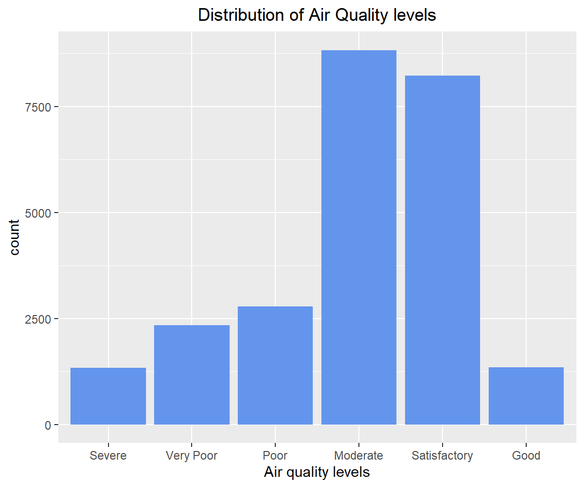

# Using treemap, let's visualize Air quality status
# install.packages('treemapify')
library(dplyr)

## 
## Attaching package: 'dplyr'

## The following objects are masked from 'package:stats':
## 
##     filter, lag

## The following objects are masked from 'package:base':
## 
##     intersect, setdiff, setequal, union

library(treemapify)

AQI_nona <- na.omit(combined[, c('City', 'Date', 'AQI_Bucket')])

treedata <- AQI_nona %>%
                count(AQI_Bucket)

ggplot(treedata, aes(fill = AQI_Bucket, area = n, label = AQI_Bucket)) +
    geom_treemap(show.legend = FALSE) +
    geom_treemap_text(colour='white', place='centre') +
    labs(title='Air quality levels') +
    theme(plot.title = element_text(hjust=0.5))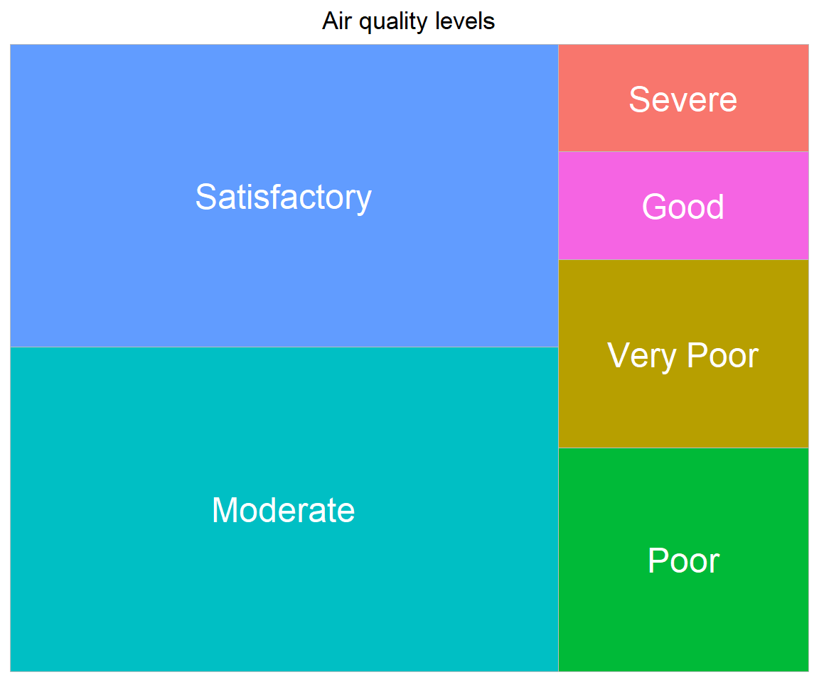

As different pollutants are measured on different scales and their range of values are fluctuating, it is important that we scale their values so that they can be brought under a common range and can be compared with each other in the same visualization.

How is Scaling/Normalization different from Standardization?

Scaling doesn’t change the distribution but only changes the range of values. Whereas Standardization is a technique used to normalize underlying distrbution so that machine learning algorithms / statistical tests which assumes data to be normal can be applied.

In our case, let’s scale our pollutant measurements to the range of 0 to 1. This process makes comparison easy and also helps us in plotting all the pollutants in a single chart to see the changes over the years. The downside of this technique in contrast to Standardization is we will end up with smaller standard deviations which can suppress the effect of outliers.

There are lot of scaling techniques available for use. In our case, let’s use MinMax Scaler.

MinMax Scaler:

Retains the shape of the original distribution
Doesn’t change the information in the data
Doesn’t effect outliers
The default range is 0 to 1

Scaling our data

Each pollutant measurement is brought to a common scale of 0 to 1 so that comparison would make sense.

pollutants <- c('PM2.5', 'PM10', 'NO', 'NO2', 'NOx', 'NH3', 'CO', 'SO2', 'O3', 'Benzene', 'Toluene', 'Xylene')


# Copy combined dataset to a new dataframe
scaled_data <- combined

# Get min value from each pollutant column
getMin <- c()
for (p in pollutants) {
    getMin <- c(getMin, min(scaled_data[,p], na.rm=TRUE))
}

# Get max value from each pollutant column
getMax <- c()
for (p in pollutants) {
    getMax <- c(getMax, max(scaled_data[,p], na.rm=TRUE))
}

# This code will loop through each column value to compute scaled value
for (i in 1:nrow(scaled_data)) {
    for (p in 1:length(pollutants)) {
        if (!is.na(scaled_data[i,pollutants[p]])) {
            scaled_data[i,pollutants[p]] <- (scaled_data[i,pollutants[p]] - getMin[p])/(getMax[p]-getMin[p])
        } else {
            scaled_data[i,pollutants[p]] <- NA
        }    
    }
}

summary(scaled_data[,pollutants])

##      PM2.5            PM10             NO             NO2       
##  Min.   :0.000   Min.   :0.000   Min.   :0.000   Min.   :0.000  
##  1st Qu.:0.030   1st Qu.:0.056   1st Qu.:0.014   1st Qu.:0.032  
##  Median :0.051   Median :0.096   Median :0.025   Median :0.060  
##  Mean   :0.071   Mean   :0.118   Mean   :0.045   Mean   :0.079  
##  3rd Qu.:0.085   3rd Qu.:0.150   3rd Qu.:0.051   3rd Qu.:0.104  
##  Max.   :1.000   Max.   :1.000   Max.   :1.000   Max.   :1.000  
##  NA's   :4598    NA's   :11140   NA's   :3582    NA's   :3585   
##       NOx             NH3              CO              SO2       
##  Min.   :0.000   Min.   :0.000   Min.   :0.0000   Min.   :0.000  
##  1st Qu.:0.027   1st Qu.:0.024   1st Qu.:0.0029   1st Qu.:0.029  
##  Median :0.050   Median :0.045   Median :0.0051   Median :0.047  
##  Mean   :0.069   Mean   :0.067   Mean   :0.0128   Mean   :0.075  
##  3rd Qu.:0.086   3rd Qu.:0.085   3rd Qu.:0.0082   3rd Qu.:0.078  
##  Max.   :1.000   Max.   :1.000   Max.   :1.0000   Max.   :1.000  
##  NA's   :4185    NA's   :10328   NA's   :2059     NA's   :3854   
##        O3           Benzene         Toluene          Xylene     
##  Min.   :0.000   Min.   :0.000   Min.   :0.000   Min.   :0.000  
##  1st Qu.:0.073   1st Qu.:0.000   1st Qu.:0.001   1st Qu.:0.001  
##  Median :0.120   Median :0.002   Median :0.007   Median :0.006  
##  Mean   :0.134   Mean   :0.007   Mean   :0.019   Mean   :0.018  
##  3rd Qu.:0.177   3rd Qu.:0.007   3rd Qu.:0.020   3rd Qu.:0.020  
##  Max.   :1.000   Max.   :1.000   Max.   :1.000   Max.   :1.000  
##  NA's   :4022    NA's   :5623    NA's   :8041    NA's   :18109

Standardization:

The below code normalizes our pollutant columns by subtracting mean from each value and dividing by standard deviation so that the data is normalized and takes the shape of bell curve.

# The code below standardizes the pollutant measurement data (by subracting mean and divide by standard deviation)
pollutants <- c('PM2.5', 'PM10', 'NO', 'NO2', 'NOx', 'NH3', 'CO', 'SO2', 'O3', 'Benzene', 'Toluene', 'Xylene')

# Copy pollution data to a new dataframe
standardized_data <- combined

# Compute mean of each of these pollutant columns
mean_list <- c()
for (p in pollutants) {
    mean_list <- c(mean_list, round(mean(standardized_data[,p], na.rm=TRUE),2))
}

# Compute standard deviation of each of these pollutant columns
sd_list <- c()
for (p in pollutants) {
    sd_list <- c(sd_list, round(sd(standardized_data[,p], na.rm=TRUE),2))
}

# This code will loop through each column value to compute normalized value
for (i in 1:nrow(standardized_data)) {
    for (p in 1:length(pollutants)) {
        if (!is.na(standardized_data[i,pollutants[p]])) {
            standardized_data[i,pollutants[p]] <- (standardized_data[i,pollutants[p]] - mean_list[p])/sd_list[p]
        } else {
            standardized_data[i,pollutants[p]] <- NA
        }    
    }
}

summary(standardized_data[,pollutants])

##      PM2.5             PM10              NO              NO2        
##  Min.   :-1.043   Min.   :-1.304   Min.   :-0.770   Min.   :-1.167  
##  1st Qu.:-0.597   1st Qu.:-0.683   1st Qu.:-0.524   1st Qu.:-0.687  
##  Median :-0.292   Median :-0.248   Median :-0.337   Median :-0.281  
##  Mean   : 0.000   Mean   : 0.000   Mean   : 0.000   Mean   : 0.000  
##  3rd Qu.: 0.203   3rd Qu.: 0.349   3rd Qu.: 0.104   3rd Qu.: 0.370  
##  Max.   :13.649   Max.   : 9.733   Max.   :16.372   Max.   :13.635  
##  NA's   :4598     NA's   :11140    NA's   :3582     NA's   :3585    
##       NOx              NH3               CO               SO2        
##  Min.   :-1.021   Min.   :-0.914   Min.   :-0.3233   Min.   :-0.801  
##  1st Qu.:-0.616   1st Qu.:-0.580   1st Qu.:-0.2500   1st Qu.:-0.489  
##  Median :-0.278   Median :-0.297   Median :-0.1954   Median :-0.296  
##  Mean   : 0.000   Mean   : 0.000   Mean   :-0.0002   Mean   : 0.000  
##  3rd Qu.: 0.247   3rd Qu.: 0.255   3rd Qu.:-0.1149   3rd Qu.: 0.038  
##  Max.   :13.754   Max.   :12.827   Max.   :24.9368   Max.   : 9.891  
##  NA's   :4185     NA's   :10328    NA's   :2059      NA's   :3854    
##        O3            Benzene          Toluene           Xylene      
##  Min.   :-1.590   Min.   :-0.207   Min.   :-0.436   Min.   :-0.486  
##  1st Qu.:-0.721   1st Qu.:-0.200   1st Qu.:-0.406   1st Qu.:-0.464  
##  Median :-0.168   Median :-0.140   Median :-0.287   Median :-0.331  
##  Mean   : 0.000   Mean   : 0.000   Mean   : 0.000   Mean   : 0.000  
##  3rd Qu.: 0.511   3rd Qu.:-0.013   3rd Qu.: 0.023   3rd Qu.: 0.044  
##  Max.   :10.292   Max.   :28.574   Max.   :22.341   Max.   :26.472  
##  NA's   :4022     NA's   :5623     NA's   :8041     NA's   :18109

ggplot(subset(scaled_data, Metropolitan_Area==1), aes(x=PM2.5, y=PM10, color=City)) +
    geom_point() +
    labs(title="PM2.5 Vs PM10 by City") +
    theme(plot.title = element_text(hjust=0.5))

The two variables PM2.5 and PM10 are positively and strongly correlated. There are visible outliers.

Scatter plot matrix:

Let’s visualize correlation between different pollutants using scatter plot matrix.

What is a scatter plot matrix?

A scatter plot matrix is collection of scatter plots displayed as a grid.

It is similar to correlation plot but instead of displaying correlations, displays underlying data.
Scatter plot matrix is created using ggpairs function from GGally package.

library(GGally)
library(dplyr)


corr_df <- scaled_data %>%
                select(PM2.5, PM10, CO, NOx, SO2)

ggpairs(corr_df) +
    labs(title = 'Understanding relationship between PM2.5, PM10, CO, NOx and SO2')

Except PM2.5 and PM10 rest of the pollutants plotted above have weak positive correlation among themselves Whereas PM2.5 and PM10 are strongly positively correlated above 0.8.

library(GGally)
library(dplyr)

corr_df <- scaled_data %>%
                select(Benzene, Toluene, Xylene)

ggpairs(corr_df) +
    labs(title = 'Understanding relationship between Benzene, Toluene, Xylene')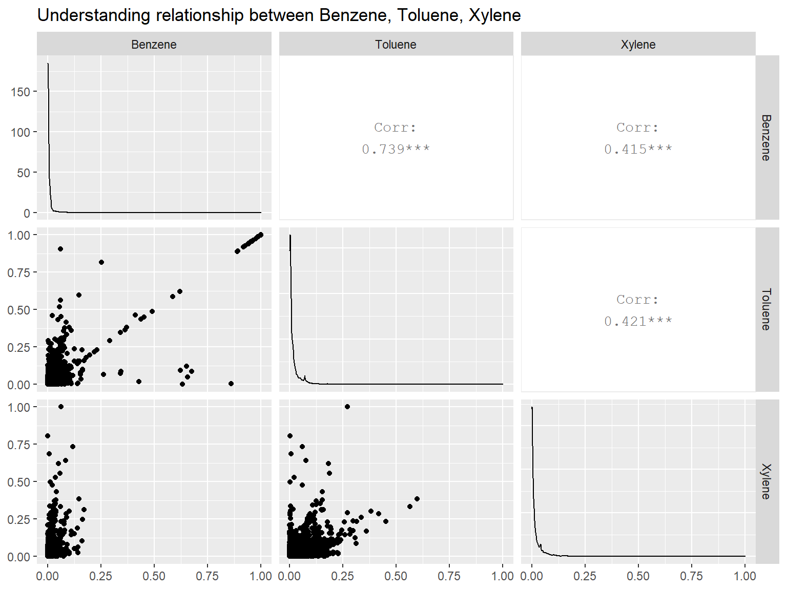

Benzene and Toluene shows somewhat stronger positive relationship correlation coefficient above 0.7.

Let’s see the distribution of pollutants over the years by City.

We will use Violin plots for this purpose.

What are Violin plots?

Violin plots are similar to kernel-density plots but are mirrored and rotated 90 degrees.

To understand more about Violin plots, check this interesting blog:

https://mode.com/blog/violin-plot-examples/

Distribution of PM2.5 by City over the years 2015-2020

# Distribution of PM2.5 by City over the years 2015-2020
ggplot(subset(scaled_data, !is.na(PM2.5)), aes(x=Date, y=PM2.5)) +
    geom_violin(color="black", fill="red") +
    facet_wrap(~City) +
    labs(title = "PM2.5 pollutant distribution by City") +
    theme(plot.title = element_text(hjust=0.5), axis.text.x = element_text(angle = 45, vjust = 0.5, hjust=1))

Cities which caught my attention with PM2.5 pollution levels close to or over 0.50: Delhi, Gurugram, Lucknow, Patna

Visible outliers found in Amritsar, Guwahati, Shillong

Let’s see how the PM2.5 pollutant is distributed by months for each year for the above cities (Delhi, Gurugram, Lucknow, Patna)

# lets see the distribution of PM2.5 by month for each year for Delhi
ggplot(subset(scaled_data, City=='Delhi' & !is.na(PM2.5)), aes(x=Month, y=PM2.5)) +
    geom_boxplot(fill="dark blue") +
    facet_wrap(~ Year, nrow=3, ncol=3) +
    labs(title="PM2.5 by month for each year - Delhi") +
    theme(plot.title = element_text(hjust=0.5))

As suspected, winter (Nov, Dec, Jan) months recorded high levels of PM2.5 for Delhi

# lets see the distribution of PM2.5 by month for each year for Gurugram
ggplot(subset(scaled_data, City=='Gurugram' & !is.na(PM2.5)), aes(x=Month, y=PM2.5)) +
    geom_boxplot(fill="red") +
    facet_wrap(~ Year, nrow=3, ncol=3) +
    labs(title="PM2.5 by month for each year - Gurugram") +
    theme(plot.title = element_text(hjust=0.5))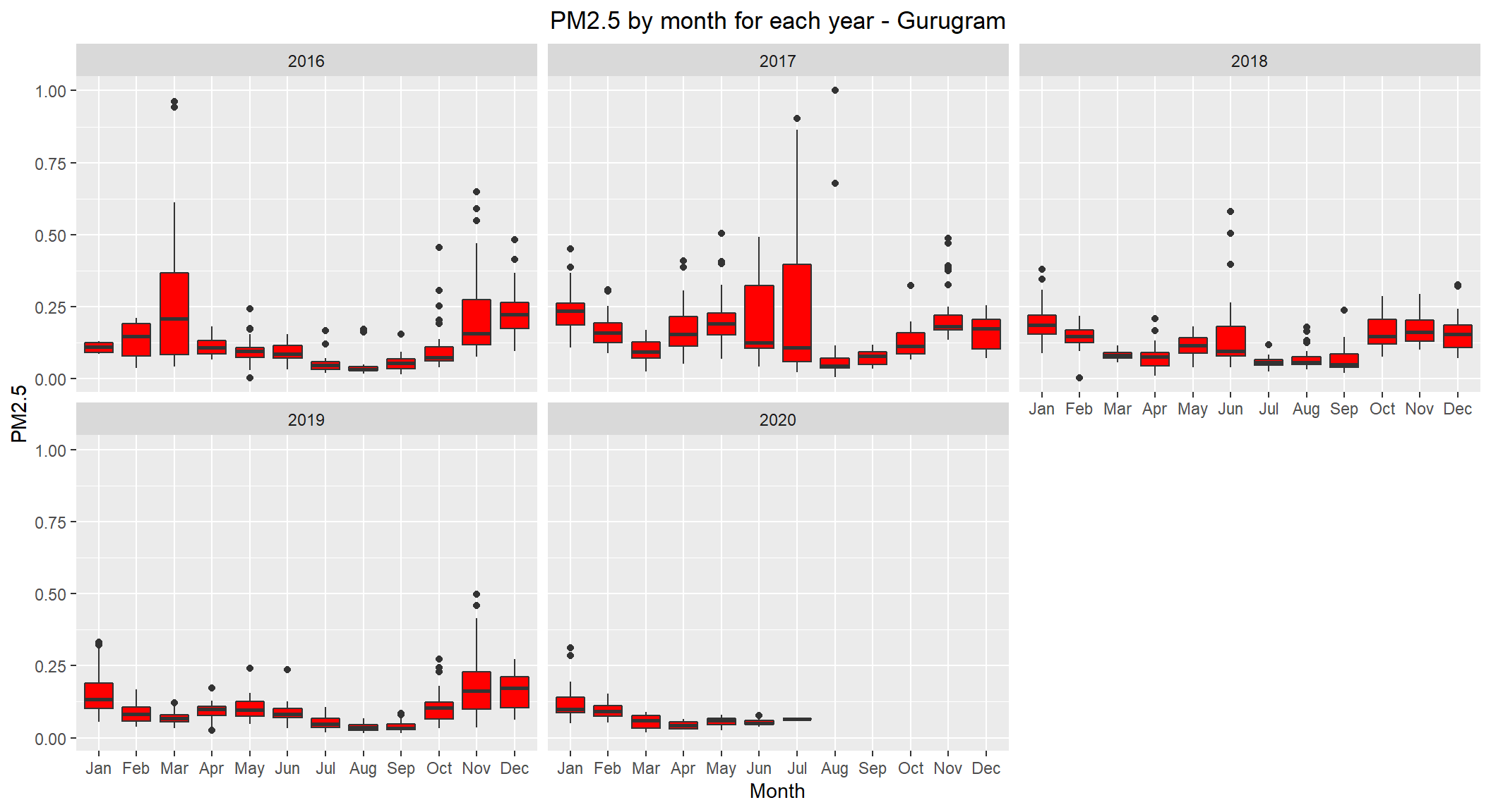

Gurugram seems to show high levels during winter. But, interestingly 2017 year showed high levels of PM2.5 during mid year.

# lets see the distribution of PM2.5 by month for each year for Lucknow
ggplot(subset(scaled_data, City=='Lucknow' & !is.na(PM2.5)), aes(x=Month, y=PM2.5)) +
    geom_boxplot(fill="cyan") +
    facet_wrap(~ Year, nrow=3, ncol=3) +
    labs(title="PM2.5 by month for each year - Lucknow") +
    theme(plot.title = element_text(hjust=0.5))

Lucknow seems to be following similar patterns as Delhi with high PM2.5 during winter.

# lets see the distribution of PM2.5 by month for each year for Patna
ggplot(subset(scaled_data, City=='Patna' & !is.na(PM2.5)), aes(x=Month, y=PM2.5)) +
    geom_boxplot(fill="yellow") +
    facet_wrap(~ Year, nrow=3, ncol=3) +
    labs(title="PM2.5 by month for each year - Patna") +
    theme(plot.title = element_text(hjust=0.5))

Patna also seems to be following similar patterns as Delhi with high PM2.5 during winter.

# PM2.5 pollutant yearly distribution for Delhi, Gurugram, Lucknow and Patna
ggplot(subset(combined, City == c('Delhi', 'Gurugram', 'Lucknow', 'Patna') & !is.na(PM2.5)), aes(x=Date, y=PM2.5)) +
    geom_boxplot(color="black", fill="pink") +
    facet_wrap(~City) +
    labs(title = "PM2.5 pollutant yearly distribution for Delhi, Gurugram, Lucknow and Patna") +
    theme(plot.title = element_text(hjust=0.5))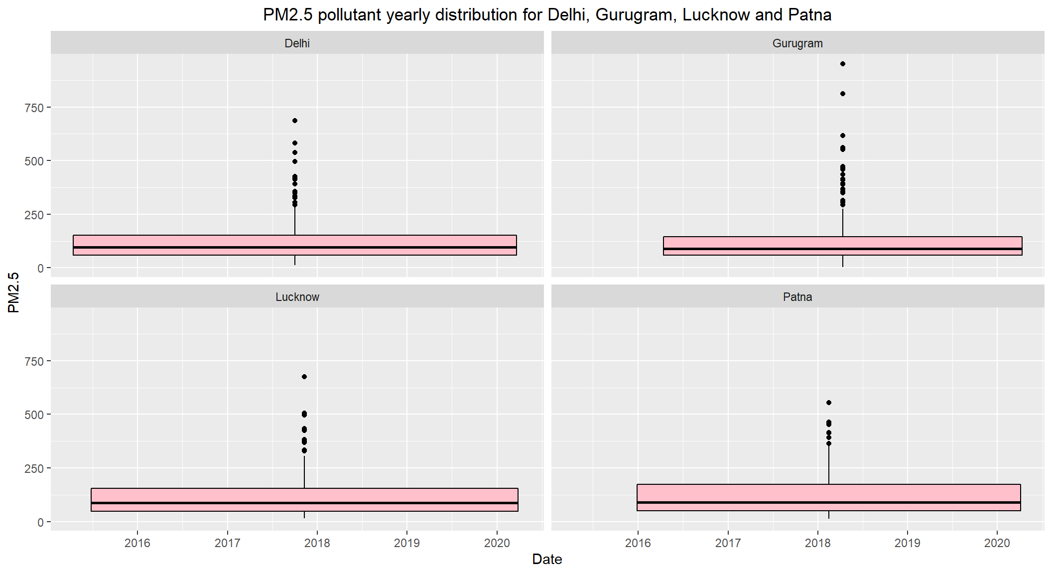

The daily permissible limits of PM2.5 is between 40 - 60
The median levels of Delhi, Gurugram, Lucknow, Patna are close to 125 which is way above the max permissible limit

Distribution of PM10 by City over the years 2015-2020

# Distribution of PM10 by City over the years 2015-2020
ggplot(subset(scaled_data, !is.na(PM10)), aes(x=Date, y=PM10)) +
    geom_violin(color="black", fill="darkblue") +
    facet_wrap(~City) +
    labs(title = "PM10 pollutant yearly distribution by City") +
    theme(plot.title = element_text(hjust=0.5))

Cities which caught my attention with PM10 levels close to and over 0.50 through the years:

Delhi, Gurugram, Jorapokhar, Kolkata, Talcher.

Interestingly metros like Bengaluru, Hyderabad seems to be consistent and median levels under 0.50 over the years.
There are visible outliers in Ahmedabad, Amritsar, Gawahati and Shillong.

Note: Jorapokhar in Jharkhand state and Talcher in Odisha state are not metro cities

Let’s see how PM10 is distributed by month over the years for the cities Delhi, Gurugram, Jorapokhar, Kolkata and Talcher

# lets see the distribution of PM10 by month for each year for Delhi
ggplot(subset(scaled_data, City=='Delhi' & !is.na(PM10)), aes(x=Month, y=PM10)) +
    geom_boxplot(fill="red") +
    facet_wrap(~ Year, nrow=3, ncol=3) +
    labs(title="PM10 by month for each year - Delhi") +
    theme(plot.title = element_text(hjust=0.5))

PM10 is also following similar patters to PM2.5 for Delhi with visible increase in levels during winter months (Nov, Dec, Jan)

# lets see the distribution of PM10 by month for each year for Gurugram
ggplot(subset(scaled_data, City=='Gurugram' & !is.na(PM10)), aes(x=Month, y=PM10)) +
    geom_boxplot(fill="cyan") +
    facet_wrap(~ Year, nrow=3, ncol=3) +
    labs(title="PM10 by month for each year - Gurugram") +
    theme(plot.title = element_text(hjust=0.5))

PM10 was recorded only for the years 2018, 2019 and 2020 for Gurugram. It is following winter pattern (with high levels during winter months) as well.

# lets see the distribution of PM10 by month for each year for Jorapokhar
ggplot(subset(scaled_data, City=='Jorapokhar' & !is.na(PM10)), aes(x=Month, y=PM10)) +
    geom_boxplot(fill="green") +
    facet_wrap(~ Year, nrow=3, ncol=3) +
    labs(title="PM10 by month for each year - Jorapokhar") +
    theme(plot.title = element_text(hjust=0.5))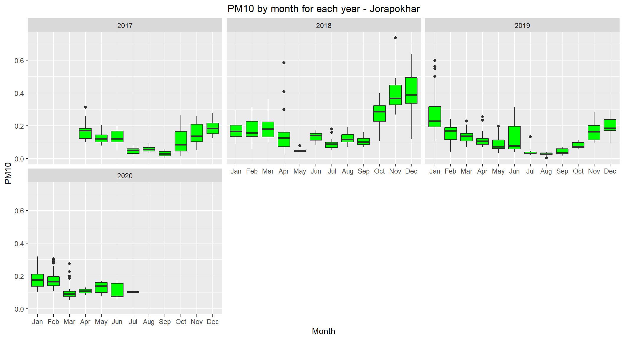

Jorapokhar is also following winter pattern (with high levels during winter months) as well.

# PM10 pollutant yearly distribution for Delhi, Gurugram, Jorapokhar, Kolkata and Talcher
ggplot(subset(combined, City == c('Delhi', 'Gurugram', 'Jorapokhar', 'Kolkata', 'Talcher') & !is.na(PM10)), aes(x=Date, y=PM10)) +
    geom_boxplot(color="black", fill="blue") +
    facet_wrap(~City) +
    labs(title = "PM10 pollutant yearly distribution for Delhi, Gurugram, Jorapokhar, Kolkata and Talcher") +
    theme(plot.title = element_text(hjust=0.5))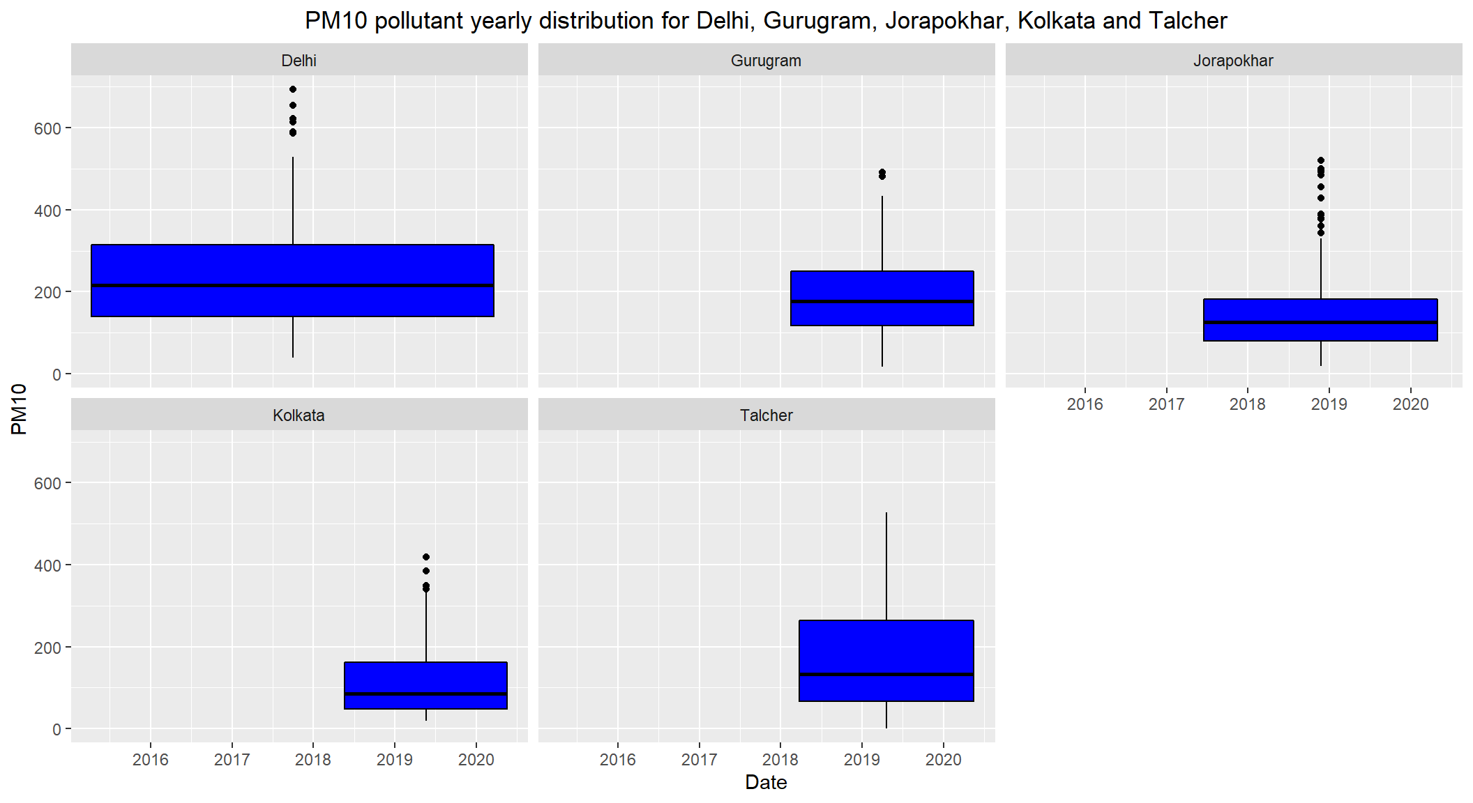

Daily permissible levels of PM10 is between 60 - 100
The median PM10 level of Delhi is over 200 which is alarming.
The median levels of Gurugram, Jorapokhar and Talcher is over 100 which is over the permissible limit
The median level of Kolkata is under and close to 100

Distribution of CO by City over the years 2015-2020

# Distribution of CO by City over the years 2015-2020
ggplot(subset(scaled_data, !is.na(CO)), aes(x=Date, y=CO)) +
    geom_violin(color="black", fill="cyan") +
    facet_wrap(~City) +
    labs(title = "CO pollutant yearly distribution by City") +
    theme(plot.title = element_text(hjust=0.5), axis.text.x = element_text(angle = 45, vjust = 0.5, hjust=1))

High CO (Carbon Monoxide) levels close to 0.50 are observed in Ahmedabad.

Let’s see the distribution of CO by month for each year for Ahmedabad

# lets see the distribution of CO by month for each year for Ahmedabad
ggplot(subset(scaled_data, City=='Ahmedabad' & !is.na(CO)), aes(x=Month, y=CO)) +
    geom_boxplot(fill="cyan") +
    facet_wrap(~ Year, nrow=3, ncol=3) +
    labs(title="CO by month for each year - Ahmedabad") +
    theme(plot.title = element_text(hjust=0.5))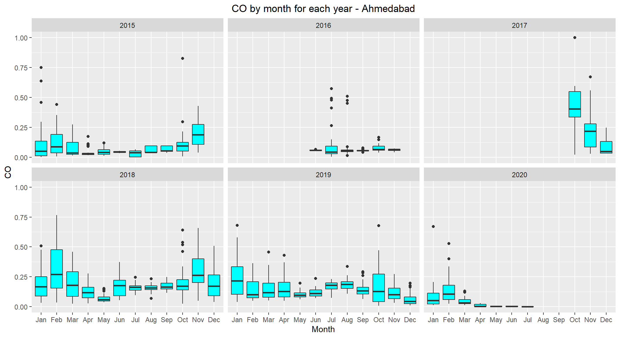

No clear visible pattern observed

# CO pollutant yearly distribution for Ahmedabad
ggplot(subset(combined, City == 'Ahmedabad' & !is.na(CO)), aes(x=Date, y=CO)) +
    geom_boxplot(color="black", fill="cyan") +
    facet_wrap(~City) +
    labs(title = "CO pollutant yearly distribution for Ahmedabad") +
    theme(plot.title = element_text(hjust=0.5))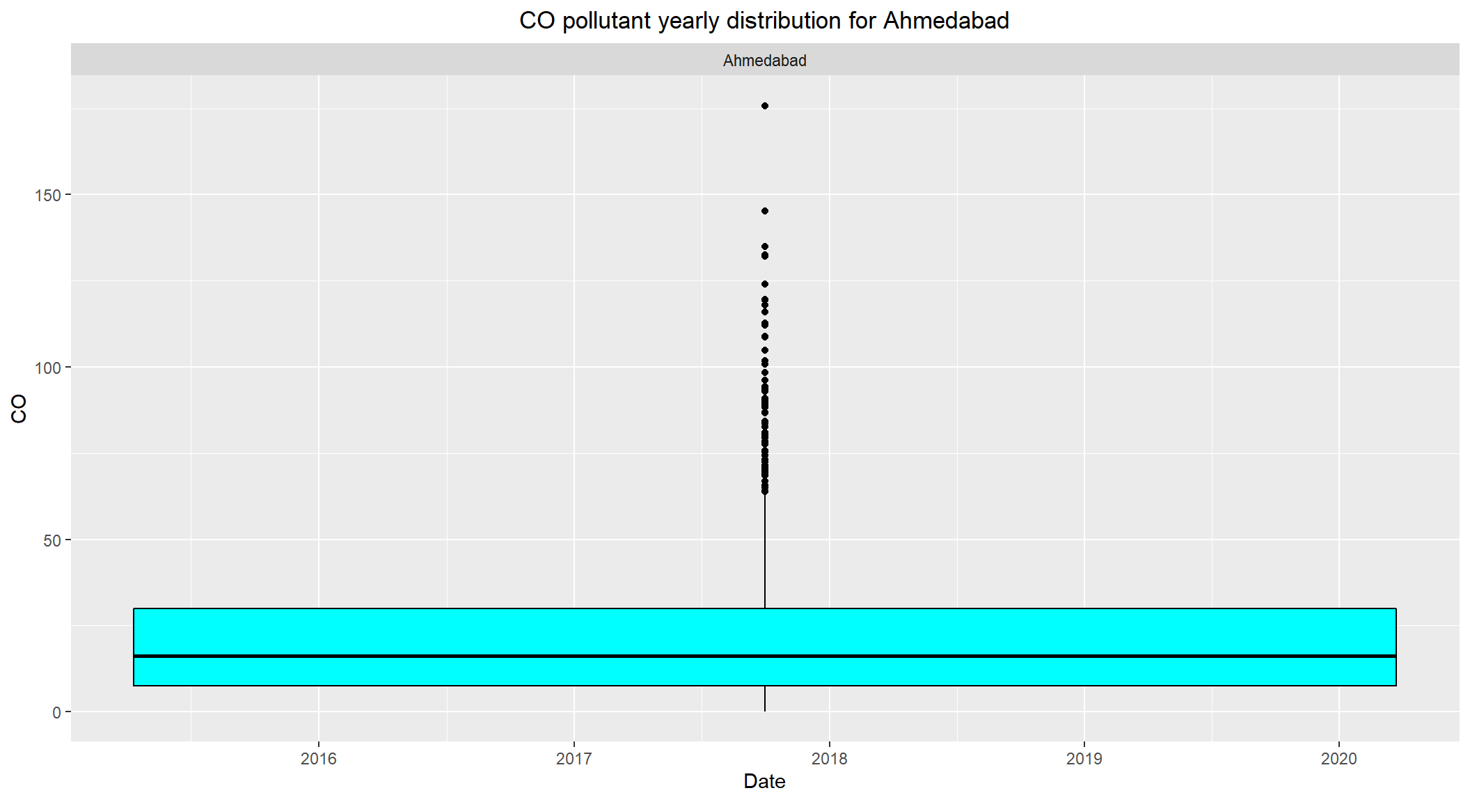

The daily permissible levels of CO is between 2 - 4
The median level of CO for Ahmedabad is over 10 which is alarming.
Visible outliers observed over 40

Distribution of NOx by City over the years 2015-2020

# Distribution of NOx by City over the years 2015-2020
ggplot(subset(scaled_data, !is.na(NOx)), aes(x=Date, y=NOx)) +
    geom_violin(color="black", fill="yellow") +
    facet_wrap(~City) +
    labs(title = "NOx pollutant yearly distribution by City") +
    theme(plot.title = element_text(hjust=0.5))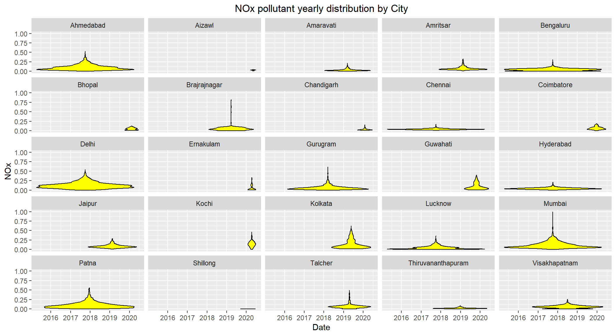

NOx levels seems to be high for Ahmedabad, Mumbai, Delhi and Patna with levels closer or over 0.50

# NOx pollutant yearly distribution for Ahmedabad, Mumbai, Delhi and Patna
ggplot(subset(combined, City == c('Ahmedabad', 'Mumbai', 'Delhi', 'Patna') & !is.na(NOx)), aes(x=Date, y=NOx)) +
    geom_boxplot(color="black", fill="yellow") +
    facet_wrap(~City) +
    labs(title = "NOx pollutant yearly distribution for Ahmedabad, Mumbai, Delhi and Patna") +
    theme(plot.title = element_text(hjust=0.5))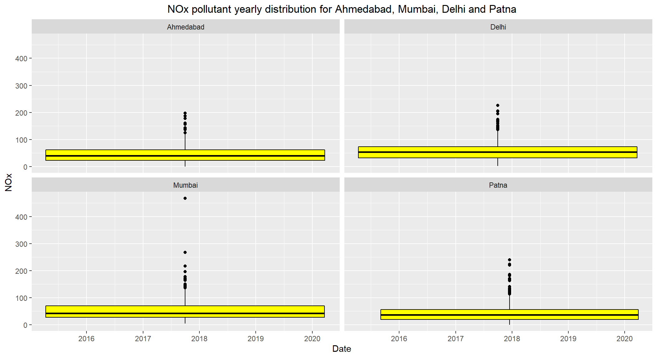

The daily permissible levels of NOx is between 40 - 80
The median levels of NOx for these cities seems to be under 80.
Visible outliers observed which are over 200

Distribution of SO2 by City over the years 2015-2020

# Distribution of SO2 by City over the years 2015-2020
ggplot(subset(scaled_data, !is.na(SO2)), aes(x=Date, y=SO2)) +
    geom_violin(color="black", fill="green") +
    facet_wrap(~City) +
    labs(title = "SO2 pollutant yearly distribution by City") +
    theme(plot.title = element_text(hjust=0.5))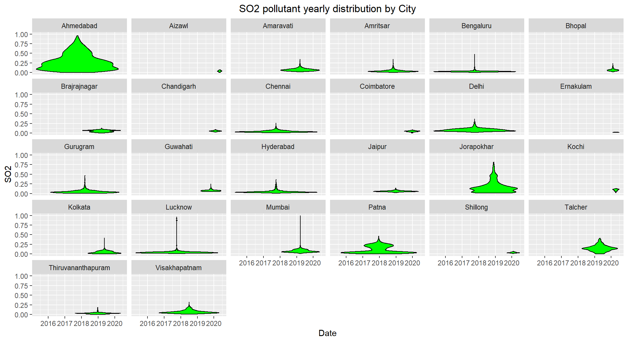

SO2 levels are high for Ahmedabad, Jorapokhar, Patna

# Distribution of SO2 over the years 2015-2020 for Ahmedabad, Jorapokhar and Patna
ggplot(subset(combined, City == c('Ahmedabad', 'Jorapokhar', 'Patna') & !is.na(SO2)), aes(x=Date, y=SO2)) +
    geom_boxplot(color="black", fill="green") +
    facet_wrap(~City) +
    labs(title = "SO2 pollutant yearly distribution for Ahmedabad, Jorapokhar and Patna") +
    theme(plot.title = element_text(hjust=0.5))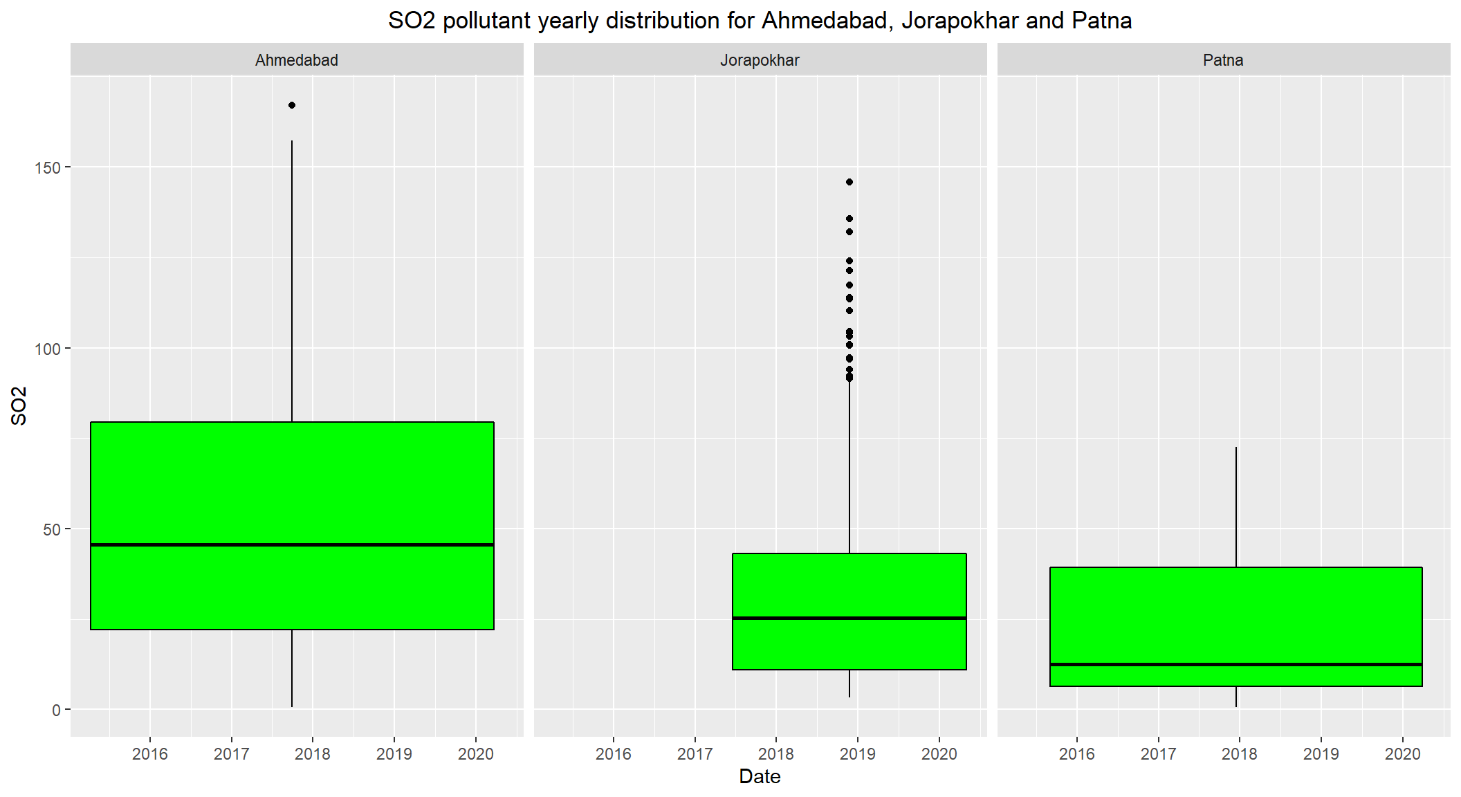

The daily permissible levels of SO2 is between 50 - 80.
Though the median levels are less than 50, it is important to keep an eye on this pollutant.
There are visible outliers recorded over 80(which is the max permissible limit).

Let’s use `plotly` to visualize PM2.5, PM10, NOx, CO and SO2 over the years

I have choosen metros Delhi, Hyderabad, Bengaluru, Chennai for indepth analysis.

Note: You may double click on the legend values to filter a particular pollutant

# Major Pollutants in Delhi over the years (2015-2020)
#install.packages("plotly")
library(dplyr)
library(plotly)

## 
## Attaching package: 'plotly'

## The following object is masked from 'package:ggplot2':
## 
##     last_plot

## The following object is masked from 'package:stats':
## 
##     filter

## The following object is masked from 'package:graphics':
## 
##     layout

del <- scaled_data %>%
        filter(City == 'Delhi')


fig <- plot_ly(del, x=~Date) %>%
        add_lines(y = ~PM2.5, name="PM2.5", visible=T) %>%
        add_lines(y = ~PM10, name="PM10", visible=T) %>%
        add_lines(y = ~NOx, name="NOx", visible=T) %>%
        add_lines(y = ~CO, name="CO", visible=T) %>%
        add_lines(y = ~SO2, name="SO2", visible=T) %>%
        layout(title = "Major pollutants in Delhi over the years (2015-2020)",
              xaxis = list(title = "Date"),
              yaxis = list(title = "Pollutant")) %>%
        config(displayModeBar=FALSE)


fig

Observations: Delhi Pollution levels

PM2.5: Clear visible peaks observed during late 2016, 2017 and 2019.
PM10: PM10 levels followed similar patterns as PM2.5. One visible peak observed during mid 2018.
NOx: Considerable peaks observed during 2015, 2016 and end of 2018
CO: Started off 2015 with high peaks and came under control during later years. One abnormal visible peak observed in Dec 2015
SO2: SO2 levels recorded high during 2016 with visible high peaks towards the end of 2016. Missing values observed during mid 2017.

library(dplyr)
library(plotly)

mum <- scaled_data %>%
        filter(City == 'Mumbai')


fig <- plot_ly(mum, x=~Date) %>%
        add_lines(y = ~PM2.5, name="PM2.5", visible=T) %>%
        add_lines(y = ~PM10, name="PM10", visible=T) %>%
        add_lines(y = ~NOx, name="NOx", visible=T) %>%
        add_lines(y = ~CO, name="CO", visible=T) %>%
        add_lines(y = ~SO2, name="SO2", visible=T) %>%
        layout(title = "Major pollutants in Mumbai over the years (2015-2020)",
              xaxis = list(title = "Date"),
              yaxis = list(title = "Pollutant")) %>%
        config(displayModeBar=FALSE)


fig

Observations: Mumbai Pollution levels

PM2.5: Peaks observed during Jan 2019 and Jan 2020.
PM10: Peaks observed during Jan 2019.
NOx: Missing values observed during the period mid 2016 till end of 2017. Abnormal peaks observed during mid 2016 before values went missing.
CO: Peaks observed during the end of 2018 and starting 2019.
SO2: No visible abnormal peaks observed. Levels seems to be consistent.

library(dplyr)
library(plotly)

hyd <- scaled_data %>%
        filter(City == 'Hyderabad')


fig <- plot_ly(hyd, x=~Date) %>%
        add_lines(y = ~PM2.5, name="PM2.5", visible=T) %>%
        add_lines(y = ~PM10, name="PM10", visible=T) %>%
        add_lines(y = ~NOx, name="NOx", visible=T) %>%
        add_lines(y = ~CO, name="CO", visible=T) %>%
        add_lines(y = ~SO2, name="SO2", visible=T) %>%
        layout(title = "Major pollutants in Hyderabad over the years (2015-2020)",
              xaxis = list(title = "Date"),
              yaxis = list(title = "Pollutant"))  %>%
        config(displayModeBar=FALSE)


fig

Observations: Hyderabad Pollution levels

PM2.5: PM2.5 levels are abnormally high during 2015 & 2016 and came under control in the subsequent years. There are visible peaks only during these years.
PM10: PM10 levels are high during winter months of each year. There is an abnormal peak during the year 2017.
NOx: NOx levels started off on a high note in 2015 but reduced gradually. There were high levels during winter and early months of 2017 till 2020 dipping during mid years.
CO: CO level seems to be high during 2015 and 2016. There is one abnormal visible peak recorded during the end of 2016. After that abnormal peak, levels seems to be low will end of 2017. From 2018, levels are more or less consistent.
SO2: SO2 levels were high from late 2016 till early 2017. From 2018, levels seems to be more or less under control.

library(dplyr)
library(plotly)

ben <- scaled_data %>%
        filter(City == 'Bengaluru')


fig <- plot_ly(ben, x=~Date) %>%
        add_lines(y = ~PM2.5, name="PM2.5", visible=T) %>%
        add_lines(y = ~PM10, name="PM10", visible=T) %>%
        add_lines(y = ~NOx, name="NOx", visible=T) %>%
        add_lines(y = ~CO, name="CO", visible=T) %>%
        add_lines(y = ~SO2, name="SO2", visible=T) %>%
        layout(title = "Major pollutants in Bengaluru over the years (2015-2020)",
              xaxis = list(title = "Date"),
              yaxis = list(title = "Pollutant"))  %>%
        config(displayModeBar=FALSE)


fig

Observations: Bengaluru Pollution Levels

PM2.5: Visible peaks observed over the years and levels seems to be high during winter of each year
PM10: PM10 levels were recorded from late 2015. PM10 levels are following similar patterns as PM2.5 with elevated levels during winter months of each year.
NOx: Looks like NOx levels were not recorded from late 2016 till late 2017. High peaks observed during early 2016. Levels dipped past early months of 2020.
CO: CO levels were high between 2015 and 2016 and largely under control after 2016 except for few inconsistent visible peaks here and there.
SO2: SO2 levels were high between 2015 to 2016 and largely under control post 2016.

library(dplyr)
library(plotly)

che <- scaled_data %>%
        filter(City == 'Chennai')


fig <- plot_ly(che, x=~Date) %>%
        add_lines(y = ~PM2.5, name="PM2.5", visible=T) %>%
        add_lines(y = ~PM10, name="PM10", visible=T) %>%
        add_lines(y = ~NOx, name="NOx", visible=T) %>%
        add_lines(y = ~CO, name="CO", visible=T) %>%
        add_lines(y = ~SO2, name="SO2", visible=T) %>%
        layout(title = "Major pollutants in Chennai over the years (2015-2020)",
              xaxis = list(title = "Date"),
              yaxis = list(title = "Pollutant"))  %>%
        config(displayModeBar=FALSE)


fig

Observations: Chennai Pollution levels

PM2.5 has been consistent over the years, on a decreasing trend from late 2019 through 2020. But occasional peaks are visible.
PM10 levels are recorded from mid 2019 for Chennai. Visible peaks are observed.
NOx levels are high from mid 2018 with a visible peak during the mid of 2018.
CO levels are bit high compared to Hyderabad and Bengaluru during 2015 and till late 2016.
SO2 levels were fluctuating over the years and recorded peaks during 2015, late 2017, early 2019 and 2020.

Learning Monk Blog